39 scatter chart in excel with labels
Creating Scatter Plot with Marker Labels - Microsoft Community Right click any data point and click 'Add data labels and Excel will pick one of the columns you used to create the chart. Right click one of these data labels and click 'Format data labels' and in the context menu that pops up select 'Value from cells' and select the column of names and click OK. Present your data in a scatter chart or a line chart Select the data that you want to plot in the line chart. Click the Insert tab, and then click Insert Line or Area Chart. Click Line with Markers. Click the chart area of the chart to display the Design and Format tabs. Click the Design tab, and then click the chart style you want to use. Click the chart title and type the text you want.
Scatter chart horizontal axis labels | MrExcel Message Board If you must use a XY Chart, you will have to simulate the effect. Add a dummy series which will have all y values as zero. Then, add data labels for this new series with the desired labels. Locate the data labels below the data points, hide the default x axis labels, and format the dummy series to have no line and no marker. Click to expand...

Scatter chart in excel with labels
how to make a scatter plot in Excel - storytelling with data Select "Scatter" from the options in the "Recommended Charts" section of your ribbon. Excel will automatically create a scatter plot for you in the same sheet as your data, using the first column of your dataset as the horizontal (X) axis, and the second column as your vertical (Y) axis. A quick note here: in creating scatter plots, a ... How to display text labels in the X-axis of scatter chart in Excel? Display text labels in X-axis of scatter chart Actually, there is no way that can display text labels in the X-axis of scatter chart in Excel, but we can create a line chart and make it look like a scatter chart. 1. Select the data you use, and click Insert > Insert Line & Area Chart > Line with Markers to select a line chart. See screenshot: 2. How to Add Labels to Scatterplot Points in Excel - Statology Step 3: Add Labels to Points. Next, click anywhere on the chart until a green plus (+) sign appears in the top right corner. Then click Data Labels, then click More Options…. In the Format Data Labels window that appears on the right of the screen, uncheck the box next to Y Value and check the box next to Value From Cells.
Scatter chart in excel with labels. Excel: labels on a scatter chart, read from array - Stack Overflow Excel: labels on a scatter chart, read from array Ask Question 0 Here I have a chart I did a right-click -> "Add labels" , and it read them from my a (H/C) row. Basically, I want it to read label values from the CO2/CH4 row instead, so they would be 0,0.5,1,2,5,10 instead. How to Change Excel Chart Data Labels to Custom Values? May 05, 2010 · The Chart I have created (type thin line with tick markers) WILL NOT display x axis labels associated with more than 150 rows of data. (Noting 150/4=~ 38 labels initially chart ok, out of 1050/4=~ 263 total months labels in column A.) It does chart all 1050 rows of data values in Y at all times. Scatter Plot Chart in Excel (Examples) | How To Create Scatter ... - EDUCBA Scatter Plot Chart is available in the Insert menu tab under the Charts section, which also has different types such as Scatter Scatter with Smooth Lines and Dotes, Scatter with Smooth Lines, Straight Line with Straight Lines under both 2D and 3D types. Where to find the Scatter Plot Chart in Excel? How To Create Scatter Chart in Excel? - EDUCBA To apply the scatter chart by using the above figure, follow the below-mentioned steps as follows. Step 1 - First, select the X and Y columns as shown below. Step 2 - Go to the Insert menu and select the Scatter Chart. Step 3 - Click on the down arrow so that we will get the list of scatter chart list which is shown below.
Scatter Plots in Excel with Data Labels Select "Chart Design" from the ribbon then "Add Chart Element" Then "Data Labels". We then need to Select again and choose "More Data Label Options" i.e. the last option in the menu. This will... How to display text labels in the X-axis of scatter chart in ... Display text labels in X-axis of scatter chart. Actually, there is no way that can display text labels in the X-axis of scatter chart in Excel, but we can create a line chart and make it look like a scatter chart. 1. Select the data you use, and click Insert > Insert Line & Area Chart > Line with Markers to select a line chart. See screenshot: How to Find, Highlight, and Label a Data Point in Excel Scatter Plot? By default, the data labels are the y-coordinates. Step 3: Right-click on any of the data labels. A drop-down appears. Click on the Format Data Labels… option. Step 4: Format Data Labels dialogue box appears. Under the Label Options, check the box Value from Cells . Step 5: Data Label Range dialogue-box appears. Labeling X-Y Scatter Plots (Microsoft Excel) Just enter "Age" (including the quotation marks) for the Custom format for the cell. Then format the chart to display the label for X or Y value. When you do this, the X-axis values of the chart will probably all changed to whatever the format name is (i.e., Age). However, after formatting the X-axis to Number (with no digits after the decimal ...
How to Create a Quadrant Chart in Excel - Automate Excel First, let's add the horizontal quadrant line. Click the " Series X values" field and select the first two values from column X Value ( F2:F3 ). Move down to the " Series Y values " field, select the first two values from column Y Value ( G2:G3 ). Under " Series name ," type Horizontal line. When finished, click " OK .". How to Make a Scatter Plot in Excel and Present Your Data Add Labels to Scatter Plot Excel Data Points. You can label the data points in the X and Y chart in Microsoft Excel by following these steps: Click on any blank space of the chart and then select the Chart Elements (looks like a plus icon). Then select the Data Labels and click on the black arrow to open More Options. Excel Charts - Scatter (X Y) Chart - Tutorials Point Step 1 − Arrange the data in columns or rows on the worksheet. Step 2 − Place the x values in one row or column, and then enter the corresponding y values in the adjacent rows or columns. Step 3 − Select the data. Step 4 − On the INSERT tab, in the Charts group, click the Scatter chart icon on the Ribbon. How to use a macro to add labels to data points in an xy ... The labels and values must be laid out in exactly the format described in this article. (The upper-left cell does not have to be cell A1.) To attach text labels to data points in an xy (scatter) chart, follow these steps: On the worksheet that contains the sample data, select the cell range B1:C6.
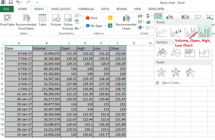
Stock chart in Excel or candlestick chart in Excel - DataScience Made Simple
Use text as horizontal labels in Excel scatter plot Edit each data label individually, type a = character and click the cell that has the corresponding text. This process can be automated with the free XY Chart Labeler add-in. Excel 2013 and newer has the option to include "Value from cells" in the data label dialog. Format the data labels to your preferences and hide the original x axis labels.

How to Add a Third Y-Axis to a Scatter Chart | EngineerExcel
Excel scatter chart using text name - Access-Excel.Tips Solution - Excel scatter chart using text name To group Grade text (ordinal data), prepare two tables: 1) Data source table 2) a mapping table indicating the desired order in X-axis In Data Source table, vlookup up "Order" from "Mapping Table", we are going to use this Order value as x-axis value instead of using Grade.

How to Make an XY Graph on Excel | Techwalla.com
Create an X Y Scatter Chart with Data Labels - YouTube How to create an X Y Scatter Chart with Data Label. There isn't a function to do it explicitly in Excel, but it can be done with a macro. The Microsoft Kno...
Example: Line Chart — XlsxWriter Documentation
How to Make a Scatter Plot in Excel | GoSkills Create a scatter plot from the first data set by highlighting the data and using the Insert > Chart > Scatter sequence. In the above image, the Scatter with straight lines and markers was selected, but of course, any one will do. The scatter plot for your first series will be placed on the worksheet. Select the chart.

How to break chart axis in Excel?
Jitter in Excel Scatter Charts • My Online Training Hub Feb 26, 2020 · Label specific Excel chart axis dates to avoid clutter and highlight specific points in time using this clever chart label trick. Jitter in Excel Scatter Charts Jitter introduces a small movement to the plotted points, making it easier to read and understand scatter plots particularly when dealing with lots of data.

Line Chart in Excel - Easy Excel Tutorial
Microsoft excel scatter plot labels - gagasscore Microsoft excel scatter plot labels In our example, we see a positive slope in the trendline indicating that the data is positively correlated. Just by looking at the trendline and the data points plotted in the scatter chart, you can get a sense of whether the data is positively correlated, negatively correlated, or not correlated.

Create a project timeline in Excel using a stacked-bar chart and data table. Milestones ar ...
Add Custom Labels to x-y Scatter plot in Excel Step 1: Select the Data, INSERT -> Recommended Charts -> Scatter chart (3 rd chart will be scatter chart) Let the plotted scatter chart be. Step 2: Click the + symbol and add data labels by clicking it as shown below. Step 3: Now we need to add the flavor names to the label. Now right click on the label and click format data labels.
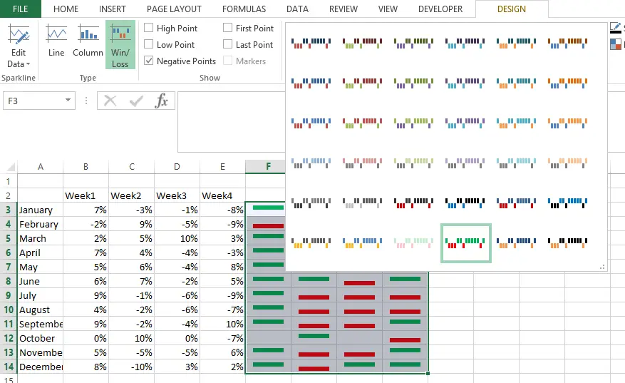
Win Loss Chart in Excel - DataScience Made Simple
How to create a scatter plot and customize data labels in Excel During Consulting Projects you will want to use a scatter plot to show potential options. Customizing data labels is not easy so today I will show you how th...
Post a Comment for "39 scatter chart in excel with labels"