40 display data labels excel
How to hide zero data labels in chart in Excel? - ExtendOffice 1. Right click at one of the data labels, and select Format Data Labels from the context menu. See screenshot: 2. In the Format Data Labels dialog, Click Number in left pane, then select Custom from the Category list box, and type #"" into the Format Code text box, and click Add button to add it to Type list box. See screenshot: 3. Data Analysis in Excel (In Easy Steps) - Excel Easy 2 Filter: Filter your Excel data if you only want to display records that meet certain criteria. 3 Conditional Formatting: ... Use a line chart if you have text labels, dates or a few numeric labels on the horizontal axis. 26 Pie Chart: Pie charts are used to display the contribution of each value (slice) to a total (pie). Pie charts always use one data series. 27 Bar Chart: A bar chart is the ...
How to Create Labels in Word from an Excel Spreadsheet - Online Tech Tips Select Browse in the pane on the right. Choose a folder to save your spreadsheet in, enter a name for your spreadsheet in the File name field, and select Save at the bottom of the window. Close the Excel window. Your Excel spreadsheet is now ready. 2. Configure Labels in Word.
Display data labels excel
Create Dynamic Chart Data Labels with Slicers - Excel Campus 10.02.2016 · Typically a chart will display data labels based on the underlying source data for the chart. In Excel 2013 a new feature called “Value from Cells” was introduced. This feature allows us to specify the a range that we want to use for the labels. Since our data labels will change between a currency ($) and percentage (%) formats, we need a ... Excel charts: how to move data labels to legend @Matt_Fischer-Daly . You can't do that, but you can show a data table below the chart instead of data labels: Click anywhere on the chart. On the Design tab of the ribbon (under Chart Tools), in the Chart Layouts group, click Add Chart Element > Data Table > With Legend Keys (or No Legend Keys if you prefer) Add or remove data labels in a chart - support.microsoft.com You can add data labels to show the data point values from the Excel sheet in the chart. This step applies to Word for Mac only: On the View menu, click Print Layout. Click the chart, and then click the Chart Design tab. Click Add Chart Element and select Data Labels, and then select a location for the data label option. Note: The options will differ depending on your chart type. If …
Display data labels excel. How to add data labels from different column in an Excel chart? Right click the data series in the chart, and select Add Data Labels > Add Data Labels from the context menu to add data labels. 2. Click any data label to select all data labels, and then click the specified data label to select it only in the chart. 3. Display Data Label for first & last data points [SOLVED] Re: Display Data Label for first & last data points My suggestion using a pivot table. However, data is in another layout in the "Data" sheet. When you add more data, simply refresh the pivot table (Data Sheet - Refresh). From the PivotTable Filter, select the Year you want to show on the graphs. Attached Files Change the format of data labels in a chart To get there, after adding your data labels, select the data label to format, and then click Chart Elements > Data Labels > More Options. To go to the appropriate area, click one of the four icons ( Fill & Line, Effects, Size & Properties ( Layout & Properties in Outlook or Word), or Label Options) shown here. How To Add Data Labels In Excel ~ Pvkngcchittoor Now we need to add the flavor names to the label.now right click on the label and click format data labels. To add or move data labels in a chart, you can do as below steps: Source: . Data labels are used to display source data in a chart directly. Change position of data labels. Source: . The column chart will appear.
How to add total labels to stacked column chart in Excel? - ExtendOffice 1. Create the stacked column chart. Select the source data, and click Insert > Insert Column or Bar Chart > Stacked Column. 2. Select the stacked column chart, and click Kutools > Charts > Chart Tools > Add Sum Labels to Chart. Then all total labels are added to every data point in the stacked column chart immediately. Excel Charts: Creating Custom Data Labels - YouTube In this video I'll show you how to add data labels to a chart in Excel and then change the range that the data labels are linked to. This video covers both W... Move data labels - support.microsoft.com Right-click the selection > Chart Elements > Data Labels arrow, and select the placement option you want. Different options are available for different chart types. For example, you can place data labels outside of the data points in a pie chart but not in a column chart. Office: Display Data Labels in a Pie Chart - Tech-Recipes: A Cookbook ... 3. In the Chart window, choose the Pie chart option from the list on the left. Next, choose the type of pie chart you want on the right side. 4. Once the chart is inserted into the document, you will notice that there are no data labels. To fix this problem, select the chart, click the plus button near the chart's bounding box on the right ...
How to show data label in "percentage" instead of - Microsoft Community Select Format Data Labels Select Number in the left column Select Percentage in the popup options In the Format code field set the number of decimal places required and click Add. (Or if the table data in in percentage format then you can select Link to source.) Click OK Regards, OssieMac Report abuse 8 people found this reply helpful · Format Data Labels in Excel- Instructions - TeachUcomp, Inc. 14.11.2019 · Then select the “Format Data Labels…” command from the pop-up menu that appears to format data labels in Excel. Using either method then displays the “Format Data Labels” task pane at the right side of the screen. Format Data Labels in Excel- Instructions: A picture of the “Format Data Labels” task pane in Excel. Edit titles or data labels in a chart - support.microsoft.com You can also place data labels in a standard position relative to their data markers. Depending on the chart type, you can choose from a variety of positioning options. On a chart, do one of the following: To reposition all data labels for an entire data series, click a data label once to select the data series. Add or remove data labels in a chart - support.microsoft.com Right-click the data series or data label to display more data for, and then click Format Data Labels. Click Label Options and under Label Contains, select the Values From Cells checkbox. When the Data Label Range dialog box appears, go back to the spreadsheet and select the range for which you want the cell values to display as data labels.
Excel Tips - How to show custom data labels in charts - YouTube
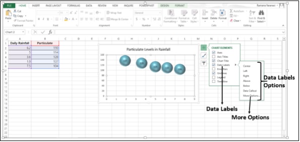
How to Add Data Labels to an Excel 2010 Chart - dummies Use the following steps to add data labels to series in a chart: Click anywhere on the chart that you want to modify. On the Chart Tools Layout tab, click the Data Labels button in the Labels group. A menu of data label placement options appears: None: The default choice; it means you don't want to display data labels. Center to position the ...
30 What Is Data Label In Excel - Labels Design Ideas 2020
Add data labels and callouts to charts in Excel 365 - EasyTweaks.com Step #3: Format the data labels. Excel also gives you the option of formatting the data labels to suit your desired look if you don't like the default. To make changes to the data labels, right-click within the chart and select the "Format Labels" option.

How to sort in Excel Tables
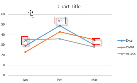
How to Change Excel Chart Data Labels to Custom Values? 05.05.2010 · Now, click on any data label. This will select “all” data labels. Now click once again. At this point excel will select only one data label. Go to Formula bar, press = and point to the cell where the data label for that chart data point is defined. Repeat the process for all other data labels, one after another. See the screencast.

How to sort data with Microsoft Excel 2016 - MATC Information Technology Programs: Degrees ...
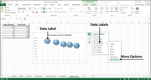
How to add or move data labels in Excel chart? - ExtendOffice 2. Then click the Chart Elements, and check Data Labels, then you can click the arrow to choose an option about the data labels in the sub menu. See screenshot: In Excel 2010 or 2007. 1. click on the chart to show the Layout tab in the Chart Tools group. See screenshot: 2. Then click Data Labels, and select one type of data labels as you need ...
Data Analysis Tool in Excel (Examples) | How To Use Data Analysis Tool?
Move data labels - support.microsoft.com Right-click the selection > Chart Elements > Data Labels arrow, and select the placement option you want. Different options are available for different chart types. For example, you can place data labels outside of the data points in a pie chart but not in a column chart.

How to create Custom Data Labels in Excel Charts - Efficiency 365
Custom Chart Data Labels In Excel With Formulas - How To Excel At Excel Follow the steps below to create the custom data labels. Select the chart label you want to change. In the formula-bar hit = (equals), select the cell reference containing your chart label's data. In this case, the first label is in cell E2. Finally, repeat for all your chart laebls.

E-xcel Tuts: Add Data Labels to Excel Charts
How to use data labels in a chart - YouTube Exceljet 41.5K subscribers 234 Dislike Share 77,351 views Oct 31, 2017 Excel charts have a flexible system to display values called "data labels". Data labels are a classic example a "simple" Excel...

How to mail merge a document
Excel tutorial: How to use data labels Generally, the easiest way to show data labels to use the chart elements menu. When you check the box, you'll see data labels appear in the chart. If you have more than one data series, you can select a series first, then turn on data labels for that series only. You can even select a single bar, and show just one data label.

E-xcel Tuts: Add Data Labels to Excel Charts
Can you display data labels on a trend line? - MrExcel Message Board Hi I have plotted some sales figures on a line chart (Jan-Aug), and added a linear trend line to view the trend to the end of the year. I have not used the 'forecast forward 4 periods' feature to do this, instead I have just selected an additional 4 blank rows below the 'august' line - which extends the x axis, and therefore extends the trend line.
Excel Charts - Free Excel Tutorial
10 spiffy new ways to show data with Excel | Computerworld 13.04.2018 · As you add data to each cell, the chart updates to display the new data. Even better, Tables bring the useful magic of Filters to your charts. Suppose you have a table with monthly budget figures ...
GNIIT HELP: Advanced Excel - Richer Data Labels ~ GNIITHELP
How to display text labels in the X-axis of scatter chart in Excel? Display text labels in X-axis of scatter chart. Actually, there is no way that can display text labels in the X-axis of scatter chart in Excel, but we can create a line chart and make it look like a scatter chart. 1. Select the data you use, and click Insert > Insert Line & Area Chart > Line with Markers to select a line chart. See screenshot:

» Excel Charts: Creating Custom Data Labels
Display Missing Dates in Excel PivotTables - My Online Training … 25.03.2014 · I use Excel 2010 and the free Power Pivot add-in, so it’s not as intuitive as Excel 2013. In order to work, you need to pull the dates from the Calendar table and then go to the PivotTable Options, click the Display tab and check the box “Show items with no data on rows”. Please test it, it should work. Thanks, Pablo

Enable or Disable Excel Data Labels at the click of a button - How To - PakAccountants.com
How to Add Data Labels in Excel - Excelchat | Excelchat In Excel 2013 and the later versions we need to do the followings; Click anywhere in the chart area to display the Chart Elements button Figure 5. Chart Elements Button Click the Chart Elements button > Select the Data Labels, then click the Arrow to choose the data labels position. Figure 6. How to Add Data Labels in Excel 2013 Figure 7.
The Stata Blog » Using import excel with real world data
Edit titles or data labels in a chart - support.microsoft.com The first click selects the data labels for the whole data series, and the second click selects the individual data label. Right-click the data label, and then click Format Data Label or Format Data Labels. Click Label Options if it's not selected, and then select the Reset Label Text check box. Top of Page
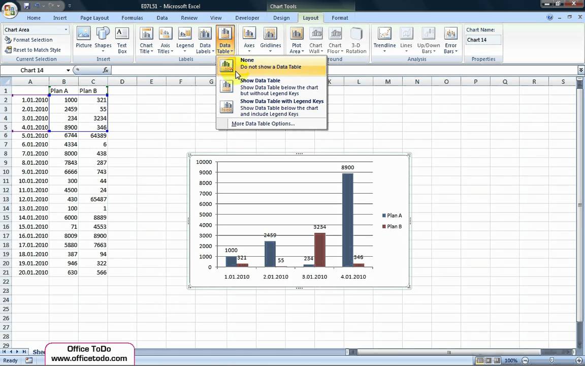
Excel | How to add a data table to a chart? - YouTube
How to add data labels from different column in an Excel chart? This method will introduce a solution to add all data labels from a different column in an Excel chart at the same time. Please do as follows: 1. Right click the data series in the chart, and select Add Data Labels > Add Data Labels from the context menu to add data labels. 2.

Multiple Series in One Excel Chart - Peltier Tech Blog
Format Data Labels in Excel- Instructions - TeachUcomp, Inc. Then select the "Format Data Labels…" command from the pop-up menu that appears to format data labels in Excel. Using either method then displays the "Format Data Labels" task pane at the right side of the screen. Set the values and positioning of the data labels in the "Label Options" category, which is shown by default.

Choosing PivotTable Layouts | Microsoft Excel - Pivot Tables
Unable to see the Label Position in excel chart. Additionally, I found a workaround for it. You can set the position of a label first, then click Label Options > Data Label Series > Clone Current Label to quickly apply custom data label formatting to the other data points in the series. Best regards, Jazlyn. -----------.
Post a Comment for "40 display data labels excel"